Peak calling
Using MACS2
For both the day 0 and day 3 of differentiation into adipocytes, two files are available
- input, as control
- histone modification H3K4
MACS2 is going to use both files to normalize the read counts and perform the peak calling.
Retrieve the BAM files with all chromosomes
cd ~/chip-seq
mkdir bams
cd bams
ln -s /scratch/users/aginolhac/chip-seq/bams/*.bam .
Perform peak calling
macs2 callpeak -t TC1-H3K4-ST2-D0.GRCm38.p3.q30.bam \
               -c TC1-I-ST2-D0.GRCm38.p3.q30.bam \
               -f BAM -g mm -n TC1-ST2-H3K4-D0 -B -q 0.01 --outdir TC1-ST2-H3K4-D0 &
macs2 callpeak -t TC1-H3K4-A-D3.GRCm38.p3.q30.bam \
               -c TC1-I-A-D3.GRCm38.p3.q30.bam \
               -f BAM -g mm -n TC1-A-H3K4-D3 -B -q 0.01 --outdir TC1-A-H3K4-D3
In case macs2 gives command not found, your are certainly missing the module, please see the set-up
check model inferred by MACS2
execute R script.
Rscript TC1-A-H3K4-D3/TC1-A-H3K4-D3_model.r
Rscript TC1-ST2-H3K4-D0/TC1-ST2-H3K4-D0_model.r
fetch the pdf produced.
sort per chromosomes and coordinates
find TC* -name '*.bdg' | parallel "sort -k1,1 -k2,2n {} > {.}.sort.bdg"
convert to bigwig
in order to get smaller files
find TC* -name '*sort.bdg' | parallel -j 2 "bedGraphToBigWig {} \
  /scratch/users/aginolhac/chip-seq/references/GRCm38.p3.chom.sizes {.}.bigwig"
Fetch the files and display them in IGV
IGV can be downloaded from the broadinstitute.
Perform peak calling with broad option
macs2 callpeak -t TC1-H3K27-ST2-D0.GRCm38.p3.q30.bam \
               -c TC1-I-ST2-D0.GRCm38.p3.q30.bam \
               -f BAM --broad -g mm -n TC1-ST2-H3K27-D0-broad -B -q 0.01 --outdir TC1-ST2-H3K27-D0-broad &
macs2 callpeak -t TC1-H3K27-A-D3.GRCm38.p3.q30.bam \
               -c TC1-I-A-D3.GRCm38.p3.q30.bam \
               -f BAM --broad -g mm -n TC1-A-H3K27-D3-broad -B -q 0.01 --outdir TC1-A-H3K27-D3-broad
Get the bigwig files for H3K27.
Redo those sort and conversion steps but only for the folders that end with 'broad'
find TC*broad -name '*.bdg' | parallel "sort -k1,1 -k2,2n {} > {.}.sort.bdg"
find TC*broad -name '*sort.bdg' | parallel -j 2 "bedGraphToBigWig {} \
  /scratch/users/aginolhac/chip-seq/references/GRCm38.p3.chom.sizes {.}.bigwig"
GREAT analysis
The website GREAT allows pasting bed regions of enriched regions.
predict functions of cis-regulatory regions
Using the TC1-A-H3K4-D3_peaks.narrowPeak file produced by MACS2.
This file has the different fields:
- chromosome
- start
- end
- peak name
- integer score for display
- strand
- fold-change
- -log10 pvalue
- -log10 qvalue
- relative summit position to peak start
Let's format the file as a 3 fields BED file and focus on more significant peaks filtering on q-values.
awk '$9>40'  TC1-A-H3K4-D3/TC1-A-H3K4-D3_peaks.narrowPeak | cut -f 1-3 | sed 's/^/chr/' >  TC1-A-H3K4-D3/TC1-A-H3K4_peaks.bed
awk '$9>40'  TC1-ST2-H3K4-D0/TC1-ST2-H3K4-D0_peaks.narrowPeak | cut -f 1-3 | sed 's/^/chr/' >  TC1-ST2-H3K4-D0/TC1-ST2-H3K4-D0_peaks.bed
For H3K27:
cat TC1-A-H3K27-D3-broad/TC1-A-H3K27-D3-broad_peaks.broadPeak | cut -f 1-3 | sed 's/^/chr/' > TC1-A-H3K27-D3-broad/TC1-A-H3K27-D3-broad_peaks.broad.bed
then
- load the BED in GREAT
- for the relevant genome,
mm10 - association rule:
- Single nearest gene for H3K4
- Two nearest genes for H3K27
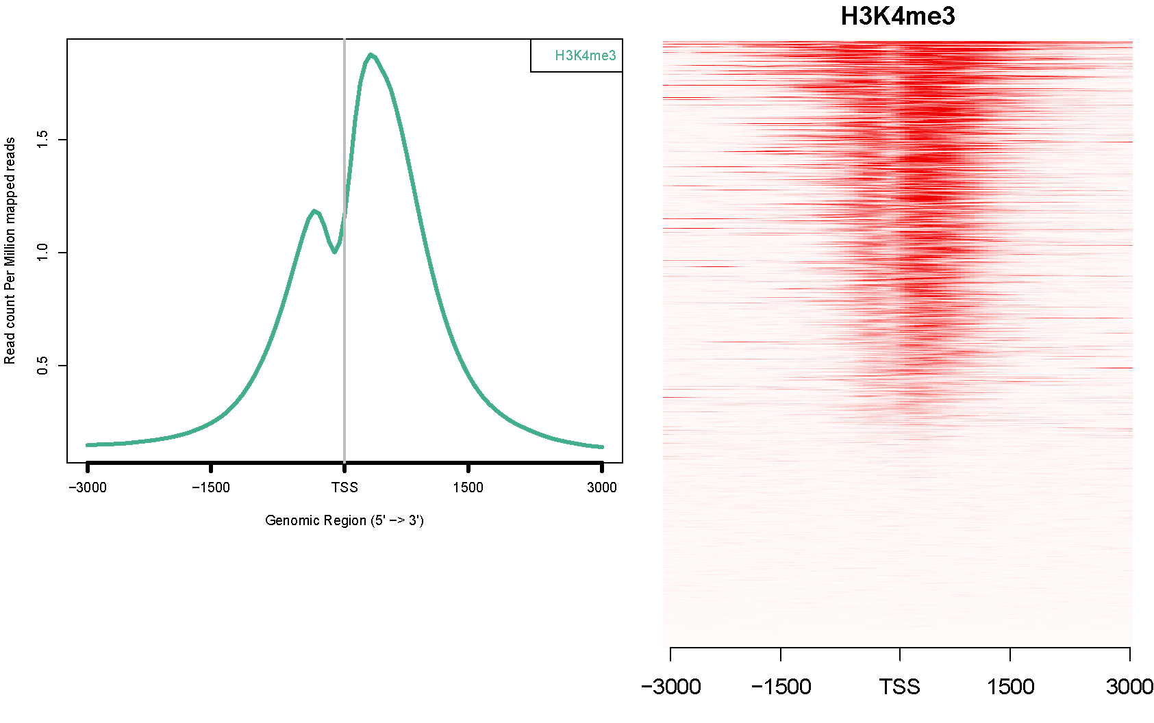
alternative with ngsplot
Example of ngsplot where gene expression ranked the genes from top to bottom and ChIP-seq of H3K4 is mapped with the red density on top.
Differential peak calling
THOR allows comparing two conditions associated with their own controls and with replicates.
- first, index the bams
parallel "samtools index {}" ::: *bam
- second, create a config file
THOR.configthat contains:
#rep1
TC1-H3K4-ST2-D0.GRCm38.p3.q30.bam
#rep2
TC1-H3K4-A-D3.GRCm38.p3.q30.bam
#chrom_sizes
/scratch/users/aginolhac/chip-seq/references/GRCm38.p3.chom.sizes
#genome
/scratch/users/aginolhac/chip-seq/references/GRCm38.p3.fasta
#inputs1
TC1-I-ST2-D0.GRCm38.p3.q30.bam
#inputs2
TC1-I-A-D3.GRCm38.p3.q30.bam
A command line looks like
rgt-THOR -m -n TC1-I-A-D0vsD3 --output-dir=TC1-I-A-D0vsD3 THOR.config
takes ~ 25 minutes
visualization
- load the file
TC1-I-A-D0vsD3-diffpeaks.bedand the bigwig files (.bwextension) - color bigwig for D0 in red
- color bigwig for D3 in green
- select both bigwig and right-click to Overlay tracks
- the BED track should display in red the regions with higher enrichments in the D0, green in the D3.
meta-analysis using GREAT
You can play with the BED file in R with this code to extract the fold-change from counts. It is encoded in the 11th field of the narrowPeak file as counts for the first condition (D0-ST2) and counts for the second condition (D3-A)
# load the file using the tidyverse
library(readr)
library(dplyr)
library(ggplot2)
library(tidyr)
diffpeaks <- read_tsv("TC1-I-A-D0vsD3-diffpeaks.bed",
                      col_names = FALSE, trim_ws = TRUE, col_types = cols(X1 = col_character()))
# split the last field into three
diffpeaks %>%
  separate(X11, into = c("count1", "count2", "third"), sep = ";", convert = TRUE) %>%
  mutate(FC = count2 / count1) -> thor_splitted
# plot the histogram of the fold-change computed above, count second condition / count 1st condition
thor_splitted %>%
  ggplot(aes(x = log2(FC))) +
  geom_histogram() +
  scale_x_continuous(breaks = seq(-5, 3, 1))

# create a bed file, append chr to chromosome names and write down the file
thor_splitted %>%
  filter(log2(FC) > 0.5) %>%
  select(X1, X2, X3) %>%
  mutate(X1 = paste0("chr", X1)) %>%
  write_tsv("THOR_logFC0.5.bed", col_names = FALSE)
you can now import the file THOR_logFC0.5.bed into GREAT and see again how the meta-analysis looks like.